Psychtoolbox-3 (PTB3)
Simple Display Calibration for Grayscale Stimuli
Using a Minolta CS100A Photometer
(Frank Schieber, University of South Dakota,
schieber@usd.edu June 13, 2007)
Abstract
This document briefly describes a set of PTB3/MATLAB scripts developed to perform simple grayscale calibration and linearization of an RGB monitor. See the built-in help and comments in each script for additional information. This code was developed and tested in a Windows environment. Mac users should be able to implement the code with little or no modification assuming that the serial I/O routines function properly (i.e., openCS100A.m, readCS100A.m and closeCS100A.m).
Click here to download zip archive containing all of the MATLAB scripts and data files described below.
Development and Test Environment
OS: Windows XP Pro (SP2)
MATLAB: 7.0.4.365 (R14) Service Pack 2
Graphics card: ATI Radeon 9600
Photometer: Minolta CS100A (Requires special cable to
connect to RS232 serial port)
Modify openCS100A/readCS100A/closeCS100A if you need to
substitute another photometer. Only luminance readings
are used here.
Files needed (over and above PTB3 distribution)
Filename Description
openCS100A.m open RS232 serial port connection to CS100A meter
readCS100A.m read luminance and chromaticity from CS100A meter
closeCS100A.m close persistent connection to CS100A meter
phase1.m collects
luminance measurements from display
using a linear gamma table
and plots results
[results saved in
phase1_photometry.mat file]
phase2.m generates
best-fit power function to the luminance
data collected by phase1.m and
then builds
an inverse gamma table to
compensate for
grayscale display
nonlinearities. Generates summary
plots and saves results in
phase2_photometry.mat
phase3.m installs inverse
gamma table generated by phase2.m
and measures screen luminance at
every possible
grayscale value [0:255].
Results are saved in
phase3_photometry.mat.
phase4.m generates a
graphical summary of all results from
calibration phases 1-3. Check
here to see how well
the inverse gamma table
succeeded in “linearizing”
the grayscale display output
Calibration procedure in a nutshell
Step 0.
The first thing that you need to do is make sure that the photometer and MATLAB can successfully communicate with one another. The Minolta CS100A photometer requires a special communications cable which plugs into the photometer at one end and a standard RS232 cable at the other end. The RS232 (serial) cable is then connected to the COM1 communications port on the computer. To coerce the CS100A to enter RS232 COMMUNICATIONS mode, you need to hold down the “F” key on the photometer while you transition the power switch from the “off” to “on” positions (A small letter “c” will appear on the LCD display to verify COMM mode). Next, execute the openCS100A script to establish a serial port connection between MATLAB and the photometer (The script returns a zero if successful). Once this connection is established, you can read the photometer as follows:
[luminance, x, y, status] = readCS100A
When finished using the photometer, good programming practice mandates that you close the serial port connection using the closeCS100A script.
Step 1.
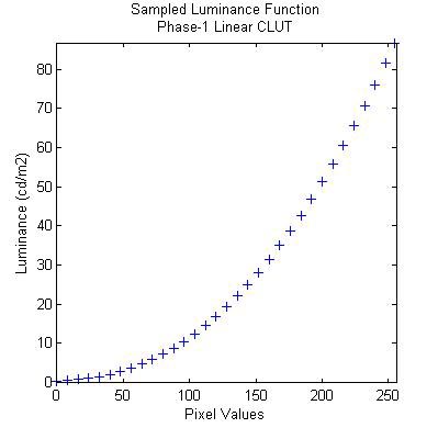
Now that you have verified a working connection to the photometer you can begin taking some preliminary measurements to characterize the photometric properties of your display system. Setup the photometer on a tripod and focus it on the display screen. Execute the phase1.m script. This script opens a PTB3 screen and prompts you to press the Enter key on the keyboard to begin. However, first you should take the opportunity to aim the photometer on the fixation point (“+”) near the center of the display. When you press the enter key, a 10 sec (default) countdown will begin to give you time to turn out the lights (and exit the room). At this point, the script generates and uploads a linear gamma table to the graphics card and then sequentially increments the luminance index of the calibration target from 0 to 255 (in steps of size 8) while the photometer collects luminance readings under program control. Feedback regarding the current index is provided in the lower left corner of the display. When the procedure is completed, a luminance-by-index curve is plotted and saved to phase1_photometry.mat (see Figure 1).
Figure 1. Sample output from phase1.m script.
Step 2.
Now that you have characterized the nonlinearity that exists between a linear
gamma table in your display adapter and the actual luminance output, you can
execute the phase2.m script to generate a best fitting power function to
the observed luminance values and then use the resulting parameters to build an
inverse gamma table1 to “linearize” the luminance output of your
display. The results of this process are summarized in a MATLAB plot and saved
to phase2_photometry.mat
(See Figures 2 and 3).
1 As currently implemented, the phase2.m script does not double-check the inverse gamma table for violations of monotonicity.
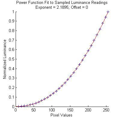
Figure 2. Best-fit power function to luminance data collected with linear gamma table.
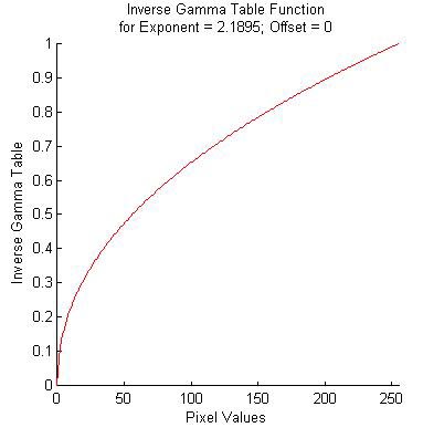
Figure 3.
Inverse gamma table generated by phase2.m to
compensate for non-linearity depicted in Figures 1 and 2.
Step 3.
Now that you have generated and saved an inverse gamma table designed to compensate for the luminance non-linearity revealed in steps 1-2, it’s time to load the inverse gamma table and evaluate how well it achieves its purpose. Execute phase3.m to load the inverse gamma table and collect luminance data from your display. This script has the same “look and feel” as phase1.m (described above) except that it takes much longer to run since it samples all possible index values from 0 thru 255. The results are automatically saved to phase3_photometry.mat and can be plotted by executing the phase4.m script. Figure 4 depicts an example of the output generated by phase4.m and reveals that the inverse gamma table did a reasonably good job of “linearizing” the luminance output of the display subsystem (see the long URL at the bottom of this page for Jenny Read’s “brute force” recursive technique for achieving optimal gamma table correction results).
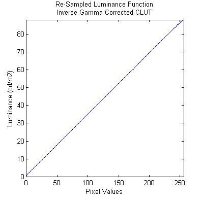
Figure 4. Linearized luminance output achieved by inverse gamma table correction.
Jenny Read’s Display Linearization Web Page (Highly
recommended)
http://www.staff.ncl.ac.uk/j.c.a.read/index.php?location=research&sub=labsetup&file=research/labsetup/gammacorrection.html